Discrete Phase Modeling
#+CATEGORY: cfd
#+TAGS: DPM ANSYS Fluent OpenFOAM Lagrangian particles multiphase reference
Introduction
The Discrete Phase Model (DPM) in ANSYS Fluent simulates a secondary phase consisting of discrete elements (such as spherical particles, aerosols, droplets, or bubbles) dispersed within a continuous fluid flow. Each element's trajectory is calculated in a Lagrangian frame of reference while simultaneously tracking associated heat transfer, mass transfer, and chemical reactions. If required, the discrete phase behavior can be fed back onto the continuous phase via source terms, establishing a bidirectional interaction between the phases.
At its core, DPM answers questions like:
- Where will particles go from this injection point?
- How does turbulence affect particle dispersion?
- How much heat is transferred between a hot gas stream and incoming droplets?
- At what rate will liquid evaporate through a particle surface?
- How will two-way coupling alter the velocity field downstream?
Discrete phase models are deployed to simulate multiphase interactions where the dispersed phase occupies a low to moderate volume fraction:
- Spray combustion:
Simulating liquid fuel sprays injected into high-temperature gas streams to model droplet trajectories and combustion rates while feeding heat and mass source terms back into the continuous gas phase.
- Cyclone separators and particle classifiers:
Simulating separation efficiency and pressure drop where strong swirl-induced centrifugal forces drive particles toward the walls for collection while clean gas exits.
- Indoor air quality and HVAC filtration:
Tracing the trajectory and deposition of fine airborne particulates through indoor spaces and ductwork, with a focus on meeting building codes that limit particulate density for human health.
- Industrial flue gas cleaning:
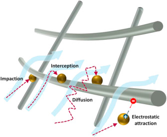
Optimizing the collection efficiency of fly ash in pollution control devices where electrostatic body forces cause fine particles to drift toward collection plates.
- Nanofluids and thermal management:
Simulating nanofluids (colloidal suspensions of ultrafine nanoparticles in a base fluid) to predict bulk thermophysical properties without relying on empirical mixture correlations. (Note: This applies to dilute mixtures; Dense Discrete Phase Models [DDPM] are required for higher concentrations).
- Medical and biomedical applications:
Simulating targeted pulmonary drug delivery within the respiratory tract, as well as tracking the evaporation, transport, and settling of bio-aerosols to evaluate isolation ward ventilation, HEPA filter locations, and air-change rates.
Key Concepts You Will Encounter
- One-Way vs Two-Way Coupling
In uncoupled (one-way) DPM, particles respond to the flow field but do not influence it. Particles exist solely for post-processing—tracing trajectories, computing deposition rates, visualizing concentration fields. In coupled (two-way or four-way) DPM, momentum, energy, and species exchange between phases modify the continuous flow solution. The choice depends on your volume fraction and the magnitude of particle-induced perturbations. See Coupling Regimes for the decision framework.
- Steady vs Unsteady Tracking
Steady tracking follows each particle from injection to escape/exit in a single pass, regardless of physical time. Unsteady tracking advances particles step-by-step in real time, updating them at the same frequency as the CFD solution. Choose steady tracking when you only care about average dispersion patterns; choose unsteady tracking when puff dynamics, pulse injection sequences, or instantaneous spatial distribution matter. See Transient DPM.
- Parcels
Because tracking individual molecules or atoms is computationally impossible, DPM groups real-world particles into "parcels" - mathematical surrogates whose collective behavior represents thousands or millions of actual particles. Each parcel carries properties (diameter, density, velocity) appropriate to a single particle, but its mass-weighted contribution scales proportionally to the physical population it represents. See
- Drag Laws
Particle acceleration depends critically on drag—the force the fluid exerts to accelerate (or decelerate) the particle toward local fluid velocity. The standard quadratic drag law works well for moderate Reynolds numbers. For accurate prediction across wide size ranges (submicron PM2.5 to millimeter droplets), you must select laws accounting for Cunningham slip correction, turbulent dispersion, and non-spherical effects. See wiki-02-fundamentals.org#drag-laws-and-response-time.
- Physical Sub-Models
DPM becomes powerful when you enable heat/mass transfer (evaporation, boiling, char combustion), Brownian motion (or UDF-defined body forces), radiation absorption, and surface interactions (wall trapping, bouncing, erosion). These sub-models determine what happens to the particle once its trajectory intersects a domain feature. See wiki-06-physical-models.org.
How DPM Relates to Other Multiphase Models
DPM sits alongside several other Euler-Lagrange and Euler-Euler approaches in the Ansys Fluent ecosystem:
- DPM
- Euler-Lagrange, dilute phases
- Sprays, aerosols, coal particles, bubble columns (low vol. fraction)
- DDPM
- Is a Hybrid Euler-Lagrange/Euler-Euler, somewhat similar to DDPM
- DPM assumes a sufficiently dilute second phase—typically below 10–12% volume fraction—and a continuum gas-phase regime (Knudsen number << 1). For higher concentrations, consider the Dense Discrete Phase Model (DDPM), which adds friction and volume-fraction effects.
- VOF
- Pure Euler-Euler
- Best suited for sharp free-surface interfaces, primary atomization. Sometimes used alongside DPM for spray simulations with a VOF-to-DPM transition that converted VOF droplets into smaller DPM droplets.
- DEM
- Pure Lagrangian, no Euler
- Solid-solid contact, packing, mechanical stress (e.g., rotating drums).
Not really fluid flow anymore, it's more solid flow with a little fluid involved.
- Mixture/Multiphase
- Euler-Euler
- Suitable for Dense suspensions, churn-turbulent regimes
Parcel Mass Scaling and the Parcel Concept
Particle Reynolds Number (Re_p) — Drag-Regime Selection Criterion
Stokes Number (Stk) — Inertia Assessment
Application: Inertial impaction deposition occurs when Stk > ~0.1 around bends, obstacles, or contractions. (See aerosols_page59.html on impaction mechanisms.)
Schmidt Number (Sc) and Sherwood Number (Sh)
Used in mass-transfer correlations (evaporation, species exchange between parcel and gas). Ranz-Marshall: =Sh = 2 + 0.6 Re_p^{1/2} Sc^{1/3}=.
Nusselt Number (Nu)
Used in convective heat transfer between parcel and gas. See #physical-models-heat-mass-transfer-and-combustion.
Summary Checklist: What You Need Before Setting Up DPM
Verify each item before opening Fluent:
- [ ] Particle diameter distribution defined (mass median aerodynamic diameter, geometric std dev)
- [ ] Particle density specified (incl. ±10% uncertainty band if measured)
- [ ] Check =Re_p~range~ → select appropriate drag law
- [ ] Compute response time τ; compare to flow time scales → choose coupling regime
- [ ] Determine if C_c correction is needed (if d < 1 μm, yes)
- [ ] Decide wall BC: trap (deposition) or escape/non-depositing
- [ ] Identify secondary forces: Brownian (d < 1 μm), Saffman lift (shear fields), thermophoresis (temperature gradients)
- [ ] Validate against analytical solution (terminal velocity, stopping distance from #fundamentals-aerosol-physics-and-drag-laws) before running coupled simulation
Governing Equation - Boussinesq-Basset-Oseen (BBO) Equation
The Boussinesq-Basset-Oseen (BBO) equation is used in Lagrangian particle tracking to describe the instantaneous motion and force balance of a small rigid spherical particle moving through a continuous fluid. It accounts for particle inertia, steady-state drag, unsteady boundary layer effects, gravity, buoyancy, and other external body forces.
Variable definitions:
| Symbol | Meaning | Typical Units |
|---|---|---|
m_p | Particle mass (πρ_p d_p³ / 6) | kg |
\mathbf{u}_p | Particle velocity vector | m/s |
\mathbf{u}(\mathbf{y},t) | Fluid velocity at particle position | m/s |
\mu | Dynamic viscosity of gas | Pa·s |
d_p | Particle diameter | m |
C_c | Cunningham slip correction factor (see below) | - |
A_p | Projected area (πd_p² / 4) | m² |
\rho_g | Gas density | kg/m³ |
\rho_p | Particle density | kg/m³ |
\mathbf{g} | Gravity vector | m/s² |
C_d | Drag coefficient (function of Re_p) | - |
For dilute, sub-micron aerosols (such as shisha PM2.5), the Stokes drag term combined with Cunningham correction and Brownian motion dominate, allowing you to safely omit the Basset history and virtual mass terms. Coupling back to the continuous phase: The total momentum extracted from or imparted to the continuous phase cell volume is calculated by summing these forces across all parcels within that cell over the integration time step.
Inertia
Represents rate of change of momentim of the particle, where $m_p$ is the particle mass and $\vec{u}_p$ is its velocity vector; dictates how the particle accelerates or decelerates in response to external forces.
Stokes Drag and Cunningham Correction
The primary viscous resistance force experienced by a particle, where $\mu$ is the fluid dynamic viscosity, $d_p$ is the particle diameter, $\vec{u}(\vec{y}(t),t)$ is the fluid velocity at the particle position $y(t)$ and at time $t$, $\vec{u}_p$ is the particle velocity, and $C_c$ is the Cunningham slip correction factor (crucial for submicron particles that don't follow continuum assumptions).
Cunningham Slip Correction Factor ($C_c$)
When particle diameter approaches the mean free path of the gas molecules, the no-slip boundary condition at the particle surface breaks down. The Cunningham slip correction factor accounts for this transition from continuum to slip-flow regime:
where Knudsen number = Kn = 2λ / d_p= and λ is the gas mean free path (~70 nm for air at STP).
Fluent implements an empirical approximation. Tabulated values for air (λ = 70 nm):
| Diameter [μm] | Kn | C_c | Regime |
|---|---|---|---|
| 10 | 0.014 | 1.018 | Continuum |
| 2 | 0.07 | 1.07 | Near-continuum |
| 1.0 | 0.14 | 1.17 | Transition start |
| 0.5 | 0.28 | 1.55 | Transition |
| 0.2 | 0.7 | 2.36 | Significant slip |
| 0.1 | 1.4 | 3.01 | Strong slip |
| 0.05 | 2.8 | 4.5+ | Free molecular approaching |
| 0.01 | 14 | 23.77 | Extreme slip |
| 0.001 | 140 | 232.5 | Free molecular |
For shisha PM2.5 (d = 0.1–2.5 μm): C_c ranges from 1.02 to 3.0. Neglecting C_c overestimates drag by 2–200%, fundamentally misrepresenting particle trajectories. Always include C_c for sub-micron work.
The Basset History Term
The Basset history integral accounts for unsteady boundary layer development around the particle.
This integral accounts for the time-dependent lag in boundary layer development around the particle when the relative velocity changes over time. However, it is computationally intensive and typically contributes very little to accuracy in turbulent gas-solid flows. Most CFD packages (ANSYS Fluent) neglect this term by default.
If you want to include it, for whatever reason, you will need to include it via a compiled UDF.
Nonlinear (Inertial) Drag
For higher particle Reynolds numbers ($Re_p > 0.5$), flow separation occurs behind the particle, introducing form drag. $C_d$ is the drag coefficient (derived from correlations like Schiller-Naumann or Haider-Levenspiel), and $A_p$ is the projected cross-sectional area ($\frac{\pi d_p^2}{4}$).
Gravity and Buoyancy
The net vertical force combining gravitational acceleration ($\mathbf{g}$) and fluid buoyancy, scaled by the density ratio between the gas ($\rho_g$) and the particle ($\rho_p$).
Additional Forces
Secondary body forces that become dominant under specific conditions:
Saffman Lift Force
Drives particles across streamlines in high-shear boundary layers.
Virtual Mass Force
Accounts for the force required to accelerate the volume of fluid surrounding the particle.
Brownian Force:
Random stochastic bombardment by gas molecules, essential for sub-micron aerosols ($d_p < 1 \, \mu m$).
Thermophoretic Force
Drives particles away from hot walls toward cooler regions under steep thermal gradients.
Relaxation Time & Particle Response
The particle relaxation time (response time) $\tau_p$ quantifies the inertia of a discrete particle relative , particularly against the fluid drag force in the low Reynolds number regime. In other words, it's how quickly a discrete particle adjusts its velocity to match the surrounding fluid.
NOTE: Add symbols table on right here
Practical Reference Table: Unit-Density Particles in Air at 1 atm, 20°C
| Diameter | Density | Terminal Velocity | Response Time |
|---|---|---|---|
| [μm] | [kg/m³] | [mm/s] | [ms] |
| 0.05 | 1000 | 0.39 | 0.04 × 10⁻³ |
| 0.1 | 1000 | 1.57 | 0.16 |
| 0.5 | 1000 | 39.2 | 4.0 |
| 1.0 | 1000 | 157 | 75.6 |
| 2.5 | 1000 | 980 | 470 |
| 5.0 | 1000 | 1,960 | 1,880 |
| 10 | 1000 | 7,470 | 3,800 |
| 20 | 1000 | 14,940 | ? |
| 50 | 1000 | ~14.9 cm/s | 7.62 ms |
Tabular data sourced from Ranz & Wong (1952), Walton & Woolcock (1960), Davies (1952).
COMMENT Key Insight
For PM2.5 (d ≤ 2.5 μm), response times range from ~0.04 ms to ~0.5 ms. Turbulent integral time scales in enclosed chambers are typically 10–100 ms. Thus St << 1 and particles track fluid closely — but for sub-micron particles (< 1 μm), additional forces (Brownian, Saffman lift, thermophoresis, van der Waals) can become dominant compared to drag. Never skip these for fine aerosol work.
Drag Laws
Each injection type defines where parcels originate in the geometry.
Creating a Single injection: 1. Select =Type=single= 2. Give name: e.g., singleInjection 3. Specify velocity: either a velocity vector (U, V, W components) OR total volumetric/gravimetric flow rate (then Fluent computes velocity based on cross-sectional area implicit in injection) 4. Set temperature 5. Set diameter — can be uniform ("monodisperse") or distribution (next section)
Creating a Surface injection: 1. Select =Type=surface= 2. Choose surface zone from list 3. Specify direction: normal, fixed vector, or inward/outward 4. Flux specification: either "volumetric flux" [=m³/(s·m²)=] or "total volume flow rate" [=m³/s=]; Fluent distributes uniformly across the surface unless specified otherwise
Creating a Conical injection: 1. Select =Type=conical= 2. Define point, cone axis, cone angle 3. Inner Angle = 0° (solid cone) or > 0° (hollow conical spray) 4. Outer Angle determines spray spread
Size Distributions
- Governing equations and parcel framework → #dpm-model-core-force-balance-and-parcels
- Deciding one-way vs two-way vs four-way coupling → #two-way-and-four-way-coupling
- Dimensionless numbers governing regimes → #fundamentals-aerosol-physics-and-drag-laws
- Brownian force UDF (required for sub-micron) → #udf-macros-and-examples
Detailed Descriptions
One-Way Coupling
The default mode in Fluent's DPM implementation. Particles follow a flow field computed independently. They do not alter it. Source terms S_{mom}, S_{energy}, S_{species} to the continuous-phase equations are set to zero.
Use when:
- Sub-micron aerosols in ventilation chambers
- Smoke/shisha PM2.5 at low emission rates
- Flow visualization with tracer particles (massless droplets or very light inert)
Two-Way Coupling
Particles impart momentum (via S_{mom}) and optionally energy/species sources back to the CFD field. Sources are computed at each coupling interval based on current parcel counts within each cell and fed to the continuous-phase solver as body-force terms.
Use when:
- Particle mass loading ratio M ≥ 0.01
- You need to capture flow modification due to heavy-laden jets
- Coal-dust cloud dynamics at moderate concentration
- Particle-laden jet mixing altering the velocity profile significantly
Four-Way Coupling
In addition to two-way momentum/energy feedback, includes inter-particle collisions modeled stochastically (O'Rourke collision kernel) alongside aerodynamic forces per parcel. Particle trajectories change due to: (a) carrier gas flow; (b) mutual drag feedback; (c) binary collisions causing momentum exchange between parcels.
Implemented by enabling:
- Two-way coupling (mandatory prerequisite)
- Stochastic collision model (from breakup/coalescence section #physical-models-heat-mass-transfer-and-combustion)
Use when:
- Spray atomization (fuel injectors, spray drying)
- Dense particulate clouds where near-field P–P collisions matter
- Erosion/glass bead blast simulations
DDPM (Eulerian-Lagrangian Dense Phase Model)
Discrete Dipole Particle Model (DDPM) extends Lagrangian parcel tracking into Eulerian granular-media territory for very high volume fractions (> ~10⁻³). It uses Kinetic Theory of Granular Flow (KTGF) to close stresses in a partially Eulerian representation while retaining Lagrangian parcel trajectories for resolved discrete elements. Suitable for dense nozzles, packed-bed reactors, and fluidized beds.
Activate in: =Models > Discrete Phase > Interaction =enable="DDPM"=. Granular temperature and pressure calculated locally within each cell based on fluctuating particle velocities approximated from kinetic theory.
Source Term Injection Mechanics
- Numerical integration choices (explicit vs implicit ODE solvers) → #fluent-setup-activation-and-configuration
- Post-processing tracks/stats/reporting methodology → #post-processing-tracks-contours-and-statistics
- Troubleshooting stuck/particle-lost/incomplete tracking failures → #validation-and-uncertainty-quantification
Particle Heat and Mass Transfer
The following heat- and mass-transfer relations apply to DPM particle models that exchange energy or species with the continuous phase.
Particle Energy Balance Equation
For a spherical parcel of diameter d_p at temperature T_p:
Terms for PM2.5 simulation:
| Symbol | Meaning | Typical significance for PM2.5 |
| -------- | --------- | ------------------------------- |
h A_p (T_g - T_p) | Convective heating/cooling from gas | **Dominant term** ✅ |
\dot{m}_{evap} h_{lv} | Latent heat of evaporation | Zero for solid inert particles ❌ |
\dot{Q}_{rad} | Net radiation exchange (P1 or DO model) | Negligible @ < 400 K; significant @ > 600 K ⚠️ |
\dot{Q}_{chem} | Exothermic/endothermic reaction enthalpy | Zero for inert soot; large for combusting fuel ❌ |
Nusselt Number Correlation (Convective Heat Transfer Coefficient)
| Regime | Nu value | Implication |
| -------- | ---------- | ------------- |
Re_p → 0 (creeping flow) | Nu ≈ 2 | Pure conduction limit (no convection enhancement) |
Moderate Re_p | Correlation increases Nu above 2 | Convection aids heat transfer |
Prandtl number =Pr = \nu/\alpha= where α is thermal diffusivity. For air at STP: ~0.71.
Sherwood Number Correlation (Convective Mass Transfer Coefficient)
Schmidt number =Sc = \nu/D= where D~binary diffusion coefficient. Used for vapor mass flux calculations during evaporation.
2. Evaporation & Boiling Laws
- Governing equations for parcel momentum/energy → #dpm-model-core-force-balance-and-parcels
- Drag law decision matrix → #fundamentals-aerosol-physics-and-drag-laws
- Source term injection mechanics → #two-way-and-four-way-coupling
- Full activation checklist + parametric study workflow → #fluent-setup-activation-and-configuration
Access: Graphics and Animations > Particle Tracks > Settings...
What You Get
After a DPM calculation completes, Fluent stores per-parcel data:
| Field | Description |
| ------- | ------------- |
Final position (x,y,z) | Last cell center or boundary face location |
Final velocity (u,v,w) | Parcel exit velocity vector |
| Diameter | Current diameter (shrinks if evaporation active) |
| Temperature | If heat-transfer model enabled |
| Status | Escaped / Trapped / Incomplete / Evaporated / Aborted |
| Residence time | Time spent in domain since injection |
| Wall impact data | Position, velocity, angle, diameter at wall contact |
All post-processing tools read from this stored data; it persists until you re-run DPM or reload a different case.
Settings Panel
| Setting | Purpose | Shisha PM2.5 recommendation |
| --------- | --------- | ---------------------------- |
| Releases | Select which injections to display | Pick your PM2.5 injection only |
| Track Particles From | All / Selected | Selected injection |
| Color by | Variable to map onto track color | Residence Time or Diameter |
| Style | Line / Sphere / Point | Line for overview; Sphere for presentations |
| Node/Cell Values | Interpolation method | Node for smooth tracks |
| Skip | Plot every Nth parcel | 50 when tracking 10 000+ parcels (reduces clutter); toggle to 1 for detail subsets |
| Coarsen | Subsample track points | 0 (full resolution) unless file-writing is bottlenecked |
| Symbol Size | Sphere diameter (if style = sphere) | Adjust to match domain scale |
Recommended Color-by Order
1. Residence Time — reveals where particles linger 2. Diameter — shows size evolution (relevant for evaporation/breakup cases) 3. Velocity Magnitude — highlights acceleration/deceleration zones 4. Particle Temperature — useful when heat transfer is active 5. Injection ID — distinguishes multiple source regions
With very large parcel counts, rendering every track overwhelms the display. Set Skip = 50 to draw ~2 % of the parcels as representative guides; set Skip = 1 when you need precise inspection on a small region of interest.
Saving Track Data
In the Particle Tracks dialog click Save ...; Fluent writes a plain-text file with columns:
Units are SI (meters, seconds, kg, Kelvin). This file can be imported back as a File Injection to replay trajectories or parsed externally with Python / MATLAB.
Animation of Transient Tracks
For transient DPM, enable Animate in the Options section of the Particle Tracks dialog, set Frame Count and Duration, then run. Fluent updates the display each time step. Export via File > Animation > Record ... as MP4, GIF, or an image sequence. Steady-state runs produce no animation; instead use Color by Residence Time and Skip to convey temporal information statically.
CFD-Post Workflow for Publication-Quality Figures
ANSYS CFD-Post handles higher-quality rendering than Fluent's built-in graphics.
Export procedure from Fluent: 1. File > Export > EnSight Case ... 2. Output Volume = ALL, Output Surface = ALL 3. Enable Write DPM Particle Data 4. Save the .case and .geo files
In CFD-Post: particles appear under Particle Tracks in the navigator. Create contours, vector plots, streamlines, iso-surfaces of particle concentration, clip planes for internal views, and LaTeX-compatible figure exports. Use Expressions to compute derived quantities such as number density.
Troubleshooting
| Symptom | Cause | Fix |
| --------- | ------- | ----- |
| Tracks all straight lines | DRW disabled | Models > Discrete Phase > Physical Models > Stochastic Tracking > Number of Tries ≥ 10 |
| Tracks not appearing | DPM did not run or injection inactive | Check Reports > Discrete Phase > Summary first |
| Missing wall impacts | Wall BC not trap/reflect | Verify boundary conditions in Chapter 4 |
2. DPM Concentration Contours
- #fluent-setup-activation-and-configuration — prerequisites for running DPM
- #two-way-and-four-way-coupling — coupling affects what you see in results
- #validation-and-uncertainty-quantification — grid independence, uncertainty quantification
- #udf-macros-and-examples — body-force hooks modify trajectories
- Course notes
me437/§Inertial Impaction and Stokes Number → #fundamentals-aerosol-physics-and-drag-laws
Three Levels of Validation
For most research workflows, Level 2 is sufficient to validate key quantities; Level 3 provides publication-grade confidence.
Extracting Simulation Data for Point Comparison
At each experimental sensor location (x_i, y_i, z_i): 1. Create a point surface (Surface > Point …) 2. Report area-weighted average DPM Concentration on that point surface 3. For number concentration, divide mass concentration by parcel mass: ~N = C_{mass} / (\rho_p \cdot \pi d_p^3 / 6)~
For area-integrated experiments (filter/sampler): create a surface matching the sampler geometry and report Surface Integral > Area-Weighted Average > DPM Concentration.
Time-Resolved Comparison (Transient Only)
If experimental data includes a time series: set up monitor points at sensor locations during the transient run (see #transient-dpm-and-puff-dynamics) and compare simulated vs. measured time series using cross-correlation (to identify time lag) and RMSE.
2. Validation Metrics
- Post-processing tools consuming these data → #post-processing-tracks-contours-and-statistics
- UDF errors and compilation failures → #udf-macros-and-examples
- Performance diagnostics → #case-study-shisha-pm25-simulation
- Course aerosol chapters
me437/§Grid-Convergence Methods → foundational texts cited therein
#+CATEGORY: cfd
#+TAGS: DPM TUI text-user-interface journal-scripting automation command-reference
#+MATURITY: growing
#+HTML_HEAD: <link rel="stylesheet" type="text/css" href="gs-styles.css">
Overview & Usage Notes
All commands below map directly to Fluent menu paths. When wrapped in (ti-menu-load-string " … ") within a journal file they execute automatically. The basic translation rule: every GUI breadcrumb =/=> becomes a space-delimited TUI path segment.
Example: GUI path Models > Discrete Phase > Interaction maps to:
Command categories (7 total):
| Category | Section | Key Commands |
| ---------- | --------- | ------------- |
Model Activation & Global Tracking Settings
Toggle DPM on/off:
define/models/discrete-phase yes— enabledefine/models/discrete-phase no— disable
Tracking modes:
define/models/discrete-phase/non-interactive— one-way (flow field frozen)define/models/discrete-phase/interactive-mode— two-way coupleddefine/models/discrete-phase/unsteady-tracking yes— transient tracking ON
Set maximum tracking steps:
- ~define/models/discrete-phase/max-steps <N>=
Activate Dense Discrete Phase Model (DDPM):
define/models/discrete-phase/dense-discrete-phase enabledefine/models/discrete-phase/dense-discrete-phase/ktgf/type algebraicdefine/models/discrete-phase/dense-discrete-phase/ktgf/type transport-equation- ~define/models/discrete-phase/dense-discrete-phase/restitution-coefficient <value>=
- ~define/models/discrete-phase/dense-discrete-phase/packing-limit <value>=
Numerics & Coupling Controls
| Command | Purpose |
| --------- | --------- |
| ~solve/set/dpm-iterations <N>= | Set total DPM iteration count |
| ~solve/set/dpm-under-relaxation <f>= | Momentum-source under-relaxation factor (default 1.0; reduce to 0.3–0.5 for stability) |
| ~solve/set/discrete-phase/coupling-interval <N>= | Couple DPM source terms every N continuous-phase iterations |
| ~solve/discrete-phase/iterations <N>= | Run N DPM iterations |
solve/discrete-phase/interaction | Iterate with full two-way coupling enabled |
solve/set/timer yes | Activate built-in profiler timer |
report/system/timer | Display wall-clock breakdown per component |
For dual-time-step (transient):
~solve/dual-time-iterate <sub-its> <steps>=
Injection Setup
Management commands:
| Command | Description |
| --------- | ------------- |
define/injections/create/single ... | Create single-point or surface injection |
define/injections/create/group ... | Create grouped injection set |
define/injections/create/file ... | Create file-based injection (import from sample) |
define/injections/create/conical ... | Conical injector type |
define/injections/create/solid-cone-atomizer ... | Solid cone spray |
define/injections/create/hollow-cone-atomizer ... | Hollow cone spray |
define/injections/create/ring ... | Ring-shaped injection |
define/injections/list | List all existing injections |
define/injections/delete | Remove an injection |
define/injections/rename | Rename an injection |
Parameters accepted via sub-commands after creating an injection (values follow in order):
type: surface / point / facex0 y0 z0— position coordinates [m]direction xdir ydir zdir— direction vectordiameter <value>— particle diameter [m]total-flow-rate <value>— mass flow rate [kg/s]number-of-parcels <value>— parcels releasedmaterial <material-name>— particle materialstart-time <value>,stop-time <value>,interval <value>— transient release schedulevelocity <value>— injection velocity [m/s]temperature <value>— injection temperature [K]size-distribution uniform— constant diameter overridesize-distribution log-normal— log-normal size distributionsize-distribution rosin-rammler— Rosin-Rammler PSDsize-distribution custom— user-defined table
Boundary Conditions
Wall zone boundary condition assignment:
| Command | Meaning |
| --------- | --------- |
define/boundary-conditions/wall/<zone>/dpm/trap | Particle absorbed / deposited |
define/boundary-conditions/wall/<zone>/dpm/escape | Particle exits domain |
define/boundary-conditions/wall/<zone>/dpm/reflect | Perfectly elastic reflect |
define/boundary-conditions/wall/<zone>/dpm/bounce | Bounce with restitution coefficients |
define/boundary-conditions/wall/<zone>/dpm/wall-jet | Wall-jet impaction model |
define/boundary-conditions/wall/<zone>/dpm/semi-reflect | Sticking-probability bounce |
define/boundary-conditions/outlet/<zone>/dpm/escape | Default outlet behaviour |
define/boundary-conditions/inlet/<zone>/dpm/reflect | Reflect inward-facing particles at inlets (useful when reversed flow is expected) |
Bounce-type restitution parameters (after selecting bounce BC):
- ~define/boundary-conditions/wall/<zone>/dpm/bounce/tangential-restitution <value>= (0–1)
- ~define/boundary-conditions/wall/<zone>/dpm/bounce/normal-rest <value>= (0–1)
Erosion/accretion reporting:
define/boundary-conditions/wall/<zone>/dpm/erosion/model finniedefine/boundary-conditions/wall/<zone>/dpm/erosion/model okadefine/boundary-conditions/wall/<zone>/dpm/erosion/model user-defined
Physical Models (Force Toggles)
All secondary-body-force toggles live under:
~define/models/discrete-phase/physical-models/<force-name>/<enable/disable>=
Specific commands:
| Toggles | Effect |
| --------- | -------- |
stochastic-tracking/enable / ~stochastic-tracking/number-of-tries <N>= | DRW dispersion |
thermophoretic-force/enable | Thermophoresis |
saffman-lift/enable | Saffman shear lift |
virtual-mass/enable | Virtual-mass body force |
pressure-gradient/enable | Pressure-gradient force |
brownian-motion/enable | Built-in Brownian toggle (v2024R1+) |
Reporting & Sampling
Global statistics and post-processing data extraction:
| Command | Output |
| --------- | -------- |
report/discrete-phase/summary | Escape/trap/incomplete counts + mass balance globally |
report/discrete-phase/injection-summary | Same metrics broken down per injection |
report/discrete-phase/sample surface:<name> file:<path>.dpm write-props:yes | Write crossing-particle sample data file |
report/discrete-phase/histogram variable:diameter bins:50 range:min:max weight:number | Property histogram on screen |
| ~report/surface-integrals/area-weighted-avg field:dpm-concentration surface:<name>= | Spatial average mass concentration on chosen surface |
Graphics display control:
display/particle-tracks— show trajectory lines in current windowdisplay/contours— colour-map concentration onto planes, iso-surfaces, wallsdisplay/vectors— vector arrow plot overlay
Each accepts standard sub-options for selecting surfaces, colour scales, number of levels, node vs. cell values, ranges (auto or manual min/max).
UDF Hookup
Register compiled UDFs for DPM use:
| Command | Purpose |
| --------- | --------- |
define/user-defined/compiled-functions compile "<filename.c>" | Compile a .c UDF file |
define/user-defined/compiled-functions load | Load compiled libudf library into session |
define/user-defined/compiled-functions unload | Free library memory |
define/models/discrete-phase/interaction/drag-law/user-defined → select <my_drag_udf_name>= | Bind UDF drag function to DPM interaction menu |
define/models/discrete-phase/physical-models/body-force/x-component/user-defined → <name>= | X-component body-force override (Brownian etc.) |
define/models/discrete-phase/physical-models/body-force/y-component/user-defined → <name>= | Y-component body-force override |
define/models/discrete-phase/physical-models/body-force/z-component/user-defined → <name>= | Z-component body-force override |
define/models/discrete-phase/physical-models/erosion-rate/user-defined → <name>= | Custom erosion wear model |
define/models/discrete-phase/physical-models/boundary-condition/user-defined → <name>= | User-defined wall-bc handler |
UDF Property Accessors
Current parcel, cell-entry, and material-law accessor macros follow. For related workflows:
- #fluent-setup-activation-and-configuration — procedural walkthrough
- #validation-and-uncertainty-quantification — troubleshooting chapter references these commands throughout
- #udf-macros-and-examples — hook registration explained in depth
Current Properties
Cell-Entry Properties (suffix _0_)
These record the state when the parcel last entered the current cell — essential for finite-difference calculations:
| Macro | Meaning |
| ------- | --------- |
| `P_DIAM0(p)` | Diameter at entry |
| `P_VEL0(p)` | Velocity at entry |
| `P_T0(p)` | Temperature at entry |
| `P_MASS0(p)` | Mass at entry |
| `P_TIME0(p)` | Time at entry |
| `P_POS0(p)` | Position at entry |
Material & Law Accessors
UDF Hook Sequence & Invocation Order
The general tracking loop for one parcel runs through these stages sequentially:
Each macro below shows its signature, parameters, return type, and a worked example.
`DEFINE_DPM_BODY_FORCE(name, p, i)` — Custom Body Force
Adds to the particle force balance. Fires every sub-step inside every traversed cell. Return force per unit mass (`m/s²`).
```c #include "udf.h"
#define BOLTZMANN 1.3806488e-23
DEFINE_DPM_BODY_FORCE(brownian_force, p, i) { real T = C_T(P_CELL(p), P_CELL_THREAD(p)); real mu = C_MU_EFF(P_CELL(p), P_CELL_THREAD(p)); real dp = P_DIAM(p); real dt = CURRENT_TIMESTEP;
real sigma = sqrt(2.0 * BOLTZMANN * T / (3.0 * PI * mu * dp * dt)); real lambda = fabs(RAND_NUMBER);
* Return Langevin white-noise acceleration component in direction i return sigma lambda / (P_MASS(p)); } ```
Register with TUI command shown in #tui-command-reference. Compile first, then select this function under Models > Discrete Phase > Physical Models > Body-Force X/Y/Z Component > user-defined.
`DEFINE_DPM_DRAG(name, p, Re)` — Custom Drag Coefficient
Override or modify the drag coefficient $C_D$. Return value is scalar $C_D$.
```c #include "udf.h"
DEFINE_DPM_DRAG(custom_schiller_naumann, p, Re) { if (Re < 0.1) return 24.0 / Re; * Stokes else if (Re < 1000.0) return (24.0 / Re) (1.0 + 0.15*pow(Re, 0.687)); * Schiller-Naumann else return 0.44; / Newton regime */ } ```
`DEFINE_DPM_BC(name, p, f, f_normal, dim)` — Custom Boundary Condition
Fires on wall contact. Return controls parcel fate:
| Constant | Effect |
| ---------- | -------- |
| `PATH_ACTIVE` | Continue tracking (specify rebound coefficients separately) |
| `PATH_ABORT` | Parcel absorbed / killed |
| `PATH_ESCAPE` | Mark parcel as escaped |
```c #include "udf.h"
DEFINE_DPM_BC(sticking_bc, p, f, f_normal, dim) { real vn = P_VEL(p)[0]*f_normal[0] + P_VEL(p)[1]*f_normal[1] + P_VEL(p)[2]*f_normal[2];
real ke = 0.5 * P_MASS(p) * (P_VEL(p)[0]*P_VEL(p)[0] + P_VEL(p)[1]*P_VEL(p)[1] + P_VEL(p)[2]*P_VEL(p)[2]);
if (ke < 1e-10) * near-zero kinetic energy return PATH_ABORT; / particle sticks permanently / else return PATH_ACTIVE; / keep tracking; restitution defined by surface BC */ } ```
`DEFINE_DPM_EROSION_RATE(name, p, f, f_normal, dim)` — Erosion Model
Returns erosion rate in `kg/(m²·s)` or a custom wear metric.
```c #include "udf.h"
DEFINE_DPM_EROSION_RATE(finnie_style_erosion, p, f, f_normal, dim) { real vi = sqrt(P_VEL(p)[0]*P_VEL(p)[0] + P_VEL(p)[1]*P_VEL(p)[1] + P_VEL(p)[2]*P_VEL(p)[2]); real alpha = acos((P_VEL(p)[0]*f_normal[0] + P_VEL(p)[1]*f_normal[1] + P_VEL(p)[2]*f_normal[2]) / MAX(vi, 1e-12));
return MAX(P_MASS(p) * vi*vi * (sin(alpha) - 0.3*sin(3.0*alpha)), 0.0); } ```
`DEFINE_DPM_INJECTION_INIT(name, I)` — Per-Parcel Initialization
One-time fire at injection time; use to randomize initial conditions.
```c #include "udf.h"
DEFINE_DPM_INJECTION_INIT(random_temp_init, I) { Thread *t = I->thread; cell_t c;
begin_c_loop(c, t) { int n; for (n = 0; n < I->nop; n++) { P_INIT_TEMP(I->p[n]) = 350.0 + 20.0*((real)rand()/(real)RAND_MAX - 0.5); } } end_c_loop(c, t) } ```
`DEFINE_DPM_LAW(name, p, ci, boiling)` — Custom Physics Law
Inject entirely new physics into the parcel lifecycle (e.g. dissolution, swelling, custom evaporation):
```c #include "udusertable.h"
DEFINE_DPM_LAW(my_custom_dissolution, p, ci, boiling) { real d = P_DIAM(p); real k_diss = 1e-6; /* dissolution rate constant [m/s] / real dt = CURRENT_TIMESTEP; real d_new = d - k_diss dt;
if (d_new <= 0.0) { P_DIAM(p) = 0.0; * mark dissolved return 0; / do not apply further laws */ }
P_DIAM(p) = d_new; * shrink accordingly return 1; / proceed to next law */ } ```
`DEFINE_DPM_SCALAR_UPDATE(name, p, ci, boiling)` — Per-Cell Scalar Update
Fire when parcel enters a new cell; useful for accumulating path-dependent quantities such as total residence time or deposition mass:
```c #include "udf.h"
DEFINE_DPM_SCALAR_UPDATE(accrue_mass, p, ci, boiling) { * Accumulate deposited mass onto cell-based field / Implementation depends on whether you want to store / / custom scalars on cells; see Fluent UDF manual for / / C_UDMI / C_UDSI accessor patterns which live outside / / the strictly DPM scope but complement it heavily. */ return; } ```
Complete Brownian Force Example (Deduplicated)
This implementation is also cross-referenced internally from #physical-models-heat-mass-transfer-and-combustion and #dpm-model-core-force-balance-and-parcels, but is kept here as the canonical single copy so there is exactly one authoritative source.
Physical background (summary)**
Brownian motion arises from molecular collisions on sub-micron particles. The Langevin equation adds white-noise acceleration term with spectral density proportional to `${k_B T}/(\pi \mu d_p \Delta t)$`. In Fluent, the built-in `define/models/discrete-phase/physical-models/brownian-motion/enable` toggle works for simple cases; for full directional control or coupled multiphysics the UDF approach provides additional flexibility including position-dependent diffusivity, non-Stokes correction factors at very high Knudsen numbers, and conditional activation based on local flow metrics. For PM2.5 specifically ($d_p$ ~sub-micron), Brownian diffusion alters trajectories measurably compared to pure-drift Stokes models in low-velocity regions like dead zones around bowl walls.
Full compilable C file:**
```c * brownian_udf.c -- ANSYS Fluent DPM Brownian force via DEFINE_DPM_BODY_FORCE *
#include "udf.h"
#ifndef BOLTZMANN #define BOLTZMANN 1.3806488e-23 /* J/K */ #endif
DEFINE_DPM_BODY_FORCE(brownian_force, p, i) { real T = C_T(P_CELL(p), P_CELL_THREAD(p)); real mu_eff = C_MU_EFF(P_CELL(p), P_CELL_THREAD(p)); real dp = P_DIAM(p); real dt = CURRENT_TIMESTEP; real sig; real lam; real mass_p = P_MASS(p);
/* Guard against NaN/infinity from bad cell lookup */ if (!isfinite(T) || !isfinite(mu_eff) || dp <= 0.0 || dt <= 0.0 || !isfinite(mass_p)) return 0.0;
* Einstein-Stokes spectral intensity sig = sqrt(2.0 BOLTZMANN * T / (3.0 * PI * mu_eff * dp * dt)); lam = fabs(RAND_NUMBER); * uniform [-1, +1] → abs gives [0, 1] *
return sig * lam / mass_p; /* acceleration in direction i (m/s^2) */ } ```
Compile steps inside Fluent: ``` define/user-defined/compiled-functions >> compile brownian_udf.c >> load libudf ```
Then register: ``` Models > Discrete Phase > Physical Models > Body-Force (X, Y, Z each select "brownian_force") ```
Common Compilation & Runtime Errors
| Error Symbol | Cause | Fix |
| -------------- | ------- | ----- |
| `error C2065: 'P_DIAM' undeclared` | Missing header files | Add both `#include "udf.h"` **and** `#include "dpm.h"` |
| `LNK2019 unresolved external` | Name mismatch between macro definition and selected hook | Ensure `DEFINE_DPM_BODY_FORCE(brownian_force, ...)` name matches EXACTLY what was typed in the selection dropdown |
| Runtime SIGSEGV at `C_T(c,t)` | Pointer references invalid/dead cell | Add guard clause before accessing cell properties: `if (NULLP(t)) return 0.0;` |
| Warning C4715: not all paths return value | Conditional logic missing fallback `return` | Add explicit `return 0.0;` as the final statement after all `if/else` branches |
| UDF compiles/load but has no effect | Hook not connected in GUI panel | Verify each axis/component explicitly lists your function via Models dialog |
| Undefined RAND_NUMBER | Random number helper unavailable without proper include chain | Include `<stdio.h>` and ensure compiler flags include `-std=c99` (Fluent default for versions ≥ v20.2) |
For more detailed diagnosis see the troubleshooting table in #validation-and-uncertainty-quantification.
See Also
- #validation-and-uncertainty-quantification -- UDF-specific error resolutions
- Full working Brownian-example also linked from #physical-models-heat-mass-transfer-and-combustion and #dpm-model-core-force-balance-and-parcels
- #tui-command-reference -- how to bind compiled functions to solver hooks
Shisha PM2.5 Case Study
This chapter collects the dedicated setup, physical-model choices, automation, and analysis guidance for the steady-state shisha PM2.5 simulation.
Summary Checklist: Secondary Forces for Shisha PM2.5
<<chapter-12-activation>>
Step-by-step \( \Rightarrow \) Fluent 2024 R1
1. Continuous phase: switch solver to Transient
- General panel \( \Rightarrow \) Time =
Transient - Set physical time step
\(\Delta t\) - Set number of time steps
2. DPM: enable transient tracking
- Models \( \Rightarrow \) Discrete Phase \( \Rightarrow \) Interaction tab
- Tracking Parameters: Unsteady Particle Tracking =
ON
3. Coupling: for two-way coupling in transient
- Coupling Interval = 1 (couple every time step)
- Use Coupled (strong coupling) if mass loading ratio > 1%
- Two-way coupling mechanics detailed in #two-way-and-four-way-coupling
4. Injections: set release schedule
- Full scheduling taxonomy below under Injection Scheduling
5. (Prerequisite checklist): verify continuous phase is converged before transitioning to transient tracking — see #fluent-setup-activation-and-configuration.
TUI equivalents
  define/models/discrete-phase/unsteady-tracking yes
  solve/set/time-step 0.001
  solve/dual-time-iterate 50 20       ; 50 sub-iterations, 20 time steps
For tracking-mode switches see also #fluent-setup-activation-and-configuration which exposes steady/transient toggles. Chapter 9 contains the complete TUI command catalog. define/models/dpm/set-tracking-mode.
Time step selection — Three constraints must hold simultaneously
Recommendation table : shisha transient
The default Lagrangian time-step factor (typically 0.1 -- 0.5 of cell transit time) is defined in #fluent-setup-activation-and-configuration and should be reduced proportionally when running unsteady tracking.
Sub-iterations per time step
For implicit solver: 5 -- 20 sub-iterations per time step ensure the nonlinear equations converge within each dt.
  solve/set/discretization-scheme ...      ; verify 2nd order
  solve/dual-time-iterate 20 100            ; 20 sub-its, 100 time steps
The dual-time-stepping methodology - pseudo-time iteration embedded inside each physical time step - is explained in Steady vs. Transient DPM above and summarized in the numerics reference ANSYS Fluent Theory Guide, Dual-Time Stepping.
Injection scheduling — Release protocols for transient DPM
Particle history tracking
In transient DPM, Fluent can record the full spatio-temporal trajectory of each parcel at every time step.
Enabling history output
  define/models/discrete-phase/sample/trajectory
  solve/set/dpm-trajectory-frequency 1   ; record every time step (default)
The frequency can be raised (e.g., 10) to reduce disk I/O; see Performance Considerations below.
Trajectory-file format
The trajectory export contains one line per parcel per time step:
Columns map to: Time [s] | Parcel-ID | x, y, z [m] | u, v, w [m/s] | d [m] | T [K].
Post-export analysis
Common downstream analysis pipelines:
- Mean-square displacement (MSD) vs. time - validates Brownian diffusivity predictions against the Smoluchowski framework in Chapter 2, Smoluchowski Coagulation
- Velocity autocorrelation function
- Animated trajectories rendered in matplotlib (Python), MATLAB, or ParaView
- Residence-time distribution extracted via #post-processing-tracks-contours-and-statistics methodology
Transient post-processing
Time-series concentration at monitor points
1. Create a point surface at the breathing-zone location(s) 2. Report Definitions \( \Rightarrow \) Volume Monitor \( \Rightarrow \) select DPM Concentration quantity 3. Fluent writes concentration vs. time to a .dat file each time step 4. Plot externally in Excel, Python (matplotlib), or Fluent's built-in Plot dialog
Cross-reference: monitor-point methodology matches #validation-and-uncertainty-quantification, which recommends sampling at sensor locations during the transient run.
Animation of transient tracks
1. Graphics \( \Rightarrow \) Animation \( \Rightarrow \) Playback 2. Object = Contours of DPM Concentration (or Particle Tracks) 3. Set Frame Interval = 10 time steps (higher values reduce frame count) 4. Play inline or Export \( \Rightarrow \) MP4, GIF, or image sequence
Animation is unavailable for steady tracking; see #post-processing-tracks-contours-and-statistics for the contrast.
Time-averaged concentration
After completing the transient run, activate Fluent's accumulated time-averaging:
solve/set/time-averaging yesFluent accumulates time-averaged fields (including DPM concentration contours) starting from the current time step onward. The time-averaged concentration after \( N \) additional steps satisfies
This enables direct comparison to steady-state predictions per the validation protocol in §Validation below.
- Note about averaging across completed transients: Fluent retains the time-averaged field across job restarts within the same session. A fresh time average requires re-enabling after reload. See #post-processing-tracks-contours-and-statistics for contour rendering details.
Coupling strategy : weak vs. strong in transient
Weak coupling (segregated)
At each time step: 1. Solve continuous phase (1 step) 2. Track all particles (1 DPM iteration) 3. Deposit DPM source terms into the continuous-phase momentum / energy / species equations 4. Advance to next time step
Weak coupling is appropriate when particle mass-loading is small. See #two-way-and-four-way-coupling for quantitative thresholds.
Strong coupling (coupled inner-loop iteration)
At each time step: 1. Solve continuous phase + DPM together in an inner iteration loop 2. Repeat until coupled residuals converge (or max inner iterations reached) 3. Advance to next time step
Strong coupling is required when:
- Mass-loading ratio exceeds approximately 5%
- DPM source terms dominate the continuous-phase equations
- Segregated (weak) coupling causes divergence
Shisha-specific recommendation
One-way coupling (current steady-state setting) remains appropriate as long as added Brownian-force UDFs, thermophoretic body forces, or evaporation sources contribute negligibly to the carrier-phase momentum budget. Escalate to two-way only if post-hoc diagnostics reveal that the flow field is changing significantly due to particle momentum exchange. See also the GPU acceleration discussion in #case-study-shisha-pm25-simulation.
Performance considerations — Cost management for transient runs
Parallel DPM (transient)
DPM tracking is embarrassingly parallel once the continuous-phase flow field is known. Fluent distributes parcels across MPI ranks automatically.
  parallel/set/dpm                              ; configure load-balancing method
  solve/set/dpm-parallel yes
For larger transient campaigns, consult #case-study-shisha-pm25-simulation for domain-decomposition best practices and expected scaling curves.
Memory footprint grows linearly with enabled history output at approximately 32 bytes per step per tracked property per parcel. Disable trajectory recording unless analytically necessary to avoid memory overflow (cf. #validation-and-uncertainty-quantification).
A representative performance budget for a 1-second shisha puff campaign on 8 cores: approximately 2 -- 8 hours wall-clock, assuming \( \Delta t = 0.001 \) s, 1000 time steps, and no trajectory recording. See the full transient performance checklist in #case-study-shisha-pm25-simulation.
Validation : transient vs steady comparison — cost-benefit gate
When experimental data exists as a time series, place virtual monitor points at sensor-location coordinates during the transient run and compare simulated vs. measured time traces using the metrics above. See #validation-and-uncertainty-quantification for formula definitions.
See Also
Primary parent ID: cfd_dpm-transient-tracking.
Full navigation map → #discrete-phase-modeling-dpm-technical-wiki.
Back to → #dpm-model-core-force-balance-and-parcels | #fluent-setup-activation-and-configuration | #two-way-and-four-way-coupling | #post-processing-tracks-contours-and-statistics | #validation-and-uncertainty-quantification | #case-study-shisha-pm25-simulation
Bibliography
@article{HAN2021100134,
title = {Advances in air filtration technologies: structure-based and interaction-based approaches},
journal = {Materials Today Advances},
volume = {9},
pages = {100134},
year = {2021},
issn = {2590-0498},
doi = {https://doi.org/10.1016/j.mtadv.2021.100134},
url = {https://www.sciencedirect.com/science/article/pii/S2590049821000047},
author = {S. Han and J. Kim and S.H. Ko},
keywords = {Air pollution, Particulate matter, Clean air, Mechanical filtration, Electrostatic filtration, Nanofiber air filter, Electret air filter},
abstract = {Intensifying air pollution has engendered growing public health concerns due to its broad and adverse effects on humanity. As a result, the development of air filtration technologies has received increased attention as a practical and promising solution. Till now, many efforts have sought to advance air filtration technologies to overcome the trade-off relationship between filtration efficiency and pressure drop. This review discusses recent progress in air filtration technology with respect to two distinct strategies, the first about optimizing filter structure and then on enhancing electrostatic interaction. Three different structure-based techniques are reviewed, including fiber morphology modification, component hybridization, and multilayer stacking, and then three interaction-based approaches that operate by imposing charge are discussed, such as induction charging, triboelectric charging, and corona charging. Furthermore, two types of active air filtration applications are comprehensively discussed as interaction-based approaches. The review concludes by discussing the current limitations and future prospects of air filtration technologies, including applications beyond air purification.}
}